


Written in July 2026. Anything that has changed since then is marked with an October update.
I lined up my four best variants of Lookout, my intraday neural network ensemble, for a final scored comparison across more than three years of walk-forward windows, and I expected a clear winner. They tied, and it took me about a day to see what that was telling me.
A walk-forward window is a small test the model has never seen: train on the days just before a date, score on the unseen stretch that follows, then roll the date forward and do it again. Do that across more than three years and you get roughly 793 separate tests per contender, all on days the model never trained on.
The result
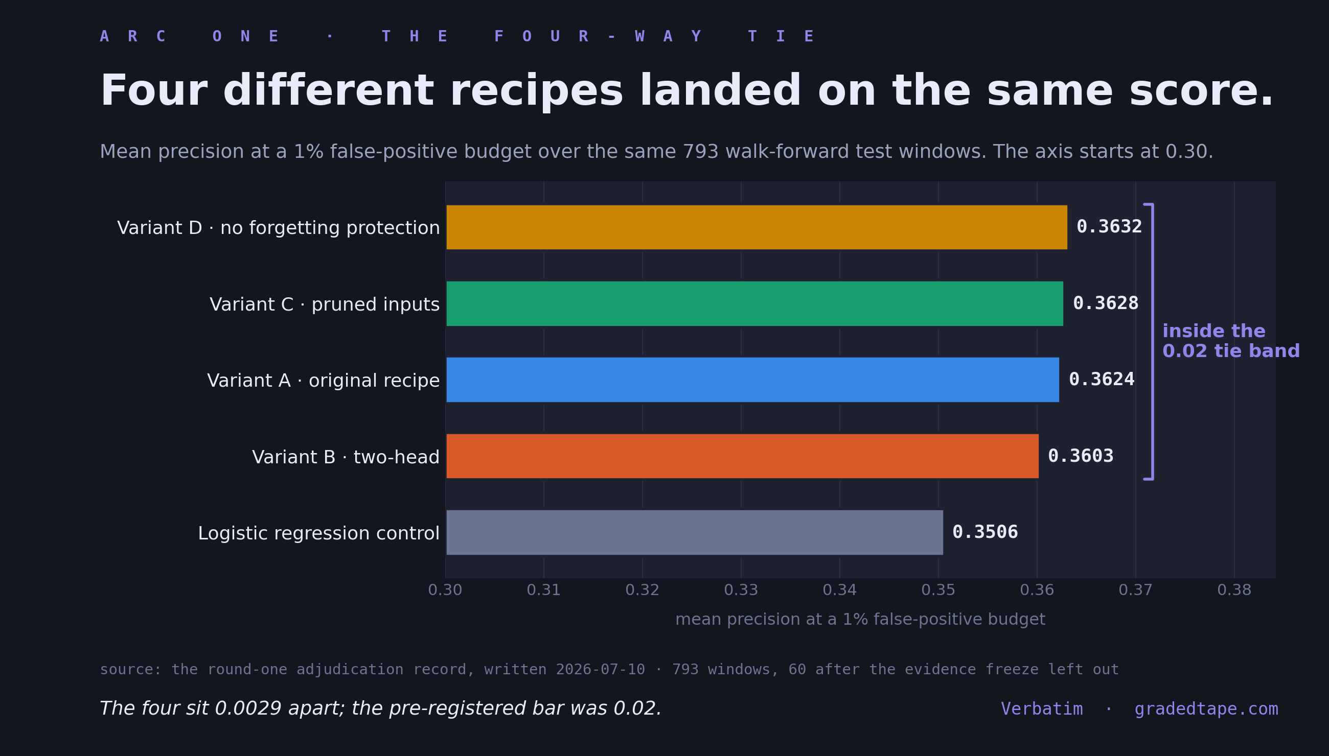
The top four are separated by three thousandths of a point on the precision statistic this program uses (the fraction of the model’s most confident flags that pay off, with false alarms held to a one percent budget). My pre-registered minimum-detectable-effect bar was 0.02, chosen in advance as roughly the smallest improvement I could reliably tell apart from window-to-window luck, and it sits nearly seven times above the largest gap among the four. Statistically, the four are the same model.
The plateau
My first reaction to the tie was disappointment. More capacity, fewer feature inputs and a more elaborate architecture all landed on the same score.
When several different attempts to be smarter all arrive at the same place, the data is telling you the bottleneck is no longer the model. Most of the signal in these feature inputs has already been found, and the useful question changes from “which architecture is best” to “what new information could I feed any of them.” That question steered the next round of research.
A lot of the good results in this notebook start out looking like failures. Subscribe to catch the next one.
Ties go to the simpler model
Under the tie-break rule that I set in advance, the win goes to Variant D, the one with an entire training-time protection mechanism removed. Fewer components at the same score is strictly better, since a deleted component can no longer fail, drift or need tuning.
The deleted mechanism protects against so-called “catastrophic forgetting” as a model retrains through time. It’s a celebrated technique in the academic literature, and I had assumed it mattered. On my data it was a no-op. Plenty of published techniques work on the benchmarks they were invented for and do nothing on a different problem, and the only way to find out is to run the boring experiment.
The logistic regression
Notice the fifth row. A plain logistic regression, roughly the simplest statistical model that could plausibly apply, gets you about 96 percent of the way to any single deep variant’s score. The remaining gap is real, and a later post in this arc asks whether it’s worth the considerable trouble. Still, if you’re a retail quant about to commit to deep learning, look at that number first. I keep the logistic regression in every comparison because it’s embarrassing.
Next
Four models that tie on average still disagree on individual days, and that disagreement is useful. The next post shows what happened when I stopped trying to break the tie and started using it. It’s the only clean win of the campaign.
Lab notebook, education and research purposes only. Not investment advice, not a solicitation; no advisory relationship is created by reading this. I trade a small account and describe my own process, errors included.
Free subscribers get the build notes below, covering eight runs on one rented GPU, and everything that broke along the way.
How I built it
All the variants ran at once on one rented H100. My model is small enough that a single card could feed eight runs, each in its own terminal session and each a flag on the same runner. A smoke test of every variant before launch caught a bug in the two-head version.